Tutorial
This is an step-by-step tutorial for SPOT analysis. If you are new to SPOT, we recommend you to follow this tutorial.
Also, if you are new to spatial perturbation analysis, we recommend you to read the following paper:
[Our paper](https://www.nature.com/articles/s41592-024-02012-z)
Preparations
Before everything, we need to prepare the data.
In this tutorial, we will use the data from [our paper](https://www.nature.com/articles/s41592-024-02012-z). The open-source data is available at [here](https://github.com/ZengLab/SPOT-paper-data).
In this set of data, we have BGI stereo-seq data of a subQ mouse MC38 tumor.
This data contains 2 files:
guide.gem: the GEM file of the guide-targeting data.
combined.h5ad: the combined AnnData object of the tissue Spatial Transcriptomics data and guide-targeting data.
Note
The guide-targeting data is the data that we used to guide the perturbation. The tissue Spatial Transcriptomics data is the data that we used to perform the spatial clustering analysis.
If you are performing SPOT analysis on your own data, you need to combine your tissue Spatial Transcriptomics data and guide-targeting data into one AnnData object also.
After downloading the data, you can check on the data by loading the AnnData object.
Note
Remember to move the data to the directory where you are running the code. Jupyter notebook is recommended for this tutorial.
import scanpy as sc
fdata = sc.read_h5ad('combined.h5ad')
fdata
You will receive the following output:
AnnData object with n_obs × n_vars = 17224 × 23376
obsm: 'spatial'
Note
The AnnData object contains the tissue Spatial Transcriptomics data and guide-targeting data. The spatial is the spatial coordinates of the data, which is used for spatial clustering analysis. The var_names is the variable names of the data, which is used for guide distribution analysis. The obs_names is the observation names of the data, which is used to contain the bin information.
More information about the AnnData object can be found at [here](https://scanpy.readthedocs.io/en/stable/api/scanpy.AnnData.html).
Importing necessary libraries
Before starting, we need to import necessary libraries.
import scanpy as sc
import squidpy as sq
import numpy as np
import matplotlib.pyplot as plt
import seaborn as sns
import pandas as pd

import sp.preprocessing as spp
SPOT required dependencies import.
Note
Import SPOT usint python, you can utilize scanpy, squidpy, numpy, matplotlib, seaborn, and pandas. scanpy and squidpy are required for spatial clustering analysis, numpy is required for numerical operations, matplotlib and seaborn are required for visualization, and pandas is required for data manipulation.
Read in the data.
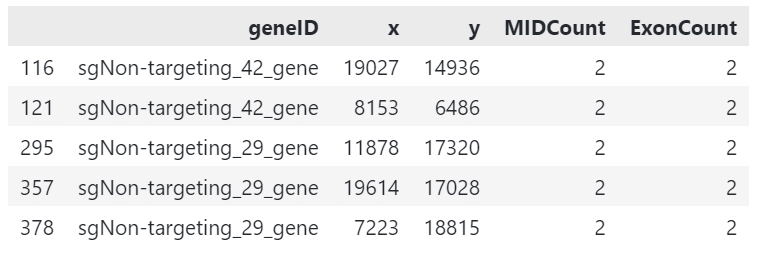
gem_df = pd.read_csv('guide.gem', sep='\t')
gem_df.head()
Preprocessing
Spatial perturbation can be highly arbitrary if we cannot perform valid preprocessing and filtering of low quality guides and bins. Refer to [our paper](https://www.nature.com/articles/s41592-024-02012-z) for our in house filtering method.
SPOT performs filtering with validation panels with the following methods.
In this tutorial we use our in house spatial transcriptomics data. This data incorporates a library of 68 guides, and is sequenced on BGI Stereo-seq platform.
# perform quality check from BGI stereo-seq GEM output
sp.preprocessing.filter_qc_bins('guide.gem')
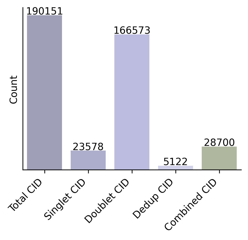
The function processes a GEM file containing guide reads and performs filtering based on the specified parameters:
Reads the GEM file and optionally filters for guides with a specific prefix
Removes bins with guide counts below the threshold if specified
Handles bins with multiple guides according to the assign_pattern:
‘max’: Keeps only the guide with highest count in each bin
‘drop’: Removes all bins that have multiple guides
‘all’: Keeps all guides in multi-guide bins
Optionally binarizes the counts (sets all to 1)
Returns filtered DataFrame or saves to file
Example usage:
filtered_data = sp.filter_guide_reads('A04091E1.gem', output_path='A04091E1_filtered.gem')
After filtering, we can perform quality control on the filtered data.
sp.preprocessing.filter_qc_bins('A04091E1_filtered.gem')

plt.figure(figsize=(8, 6))
scatter = plt.scatter(x=gdata.obsm['spatial'][:, 0], y=gdata.obsm['spatial'][:, 1],
                     s=gdata.obs['n_genes_by_counts'], alpha=0.5, c=gdata.obs['total_counts'], cmap='viridis')
sns.despine()
plt.colorbar(scatter, label='Total counts')
plt.title('Guide reads')

plt.show()

Clustering
Cluster the tissue data means finding similarity of bins in the tissue data implicating the same microenvironment.
In our case, we would like to cluster the tissue into tumor environments that could implicate different guide distribution. We can simply perform NMF clustering on the tissue data.
Attention
NMF is a simple clustering method that can be used for quick analysis. It is not recommended for complex spatial analysis.
NMF is a simple mathematical trick that can decompose the spatial expression profile into key components that we are interested in.
We apply NMF to spatial transcriptomics data. Because we want only major signals, we first filter out genes that are not significantly varied across resolution.
fdata.copy()
fdata.var["mt-"] = fdata.var_names.str.startswith("mt-")
fdata.var["gm"] = fdata.var_names.str.startswith("Gm")
fdata.var["rik"] = [True if "Rik" in str else False for str in fdata.var_names]
fdata = fdata[:, ~fdata.var["mt-"]]
fdata = fdata[:, ~fdata.var["gm"]]
fdata = fdata[:, ~fdata.var["rik"]]

with open('mouseHK.txt', 'r') as f:
    for line in f:
        hk_genes = line.split('\t')
        break
fdata = fdata[:, [gene for gene in fdata.var_names if gene not in hk_genes]]
The mouseHK.txt is a list of housekeeping genes that are derived from singlce-cell sequencing data [1].
Then we perform NMF on the filtered data with a simple function. spp.nmf_clustering()
nmf_data = spp.nmf_clustering(fdata, n_components=50)
Note
The number of components is set to 50, which is a optimal resolution of programs of genes that can be futher clustered. A larger number of components can be used for more complex analysis, but a small number is not recommended.
clustered_nmf_data = spp.nmf_consensus(nmf_data)
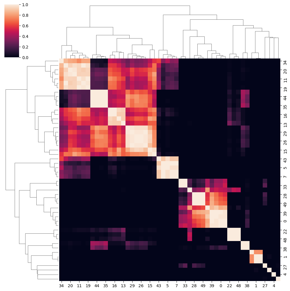
In this NMF approach, we decompose the gene expression profile space-wise into an extend of components. Then perform consensus clustering of component’s pearsonr correlation.
Then we compute the pearson correlation matrix:
Finally we perform consensus clustering on \(\mathbf{P}\).
The clustered program can then be scored using the scanpy :py:function:`tl.score_genes()` function.
The score of top optimal genes is store in the adata.obs attribute.
clustered_nmf_data.obs['nmf_cluster'] = clustered_nmf_data.obs.idxmax(axis=1).str.split('_').str[2].astype(int)
A sptial demonstration of NMF clustering is shown below.

Now that we have the clustered data, we can perform guide distribution analysis.
Cluster Dependent Analysis
In cluster dependent analysis, we perform chi-square test to determine the guide specificity in each cluster. Cluster dependent means that we would like to know the guide specificity in each cluster.
A guide’s specificity can be determined by the proportion of the guide’s reads in each cluster, and statistical significance can be determined by chi-square test.
Import the function rank_by_chi_square() to perform chi-square test.
import sp.cluster_dependent as spc
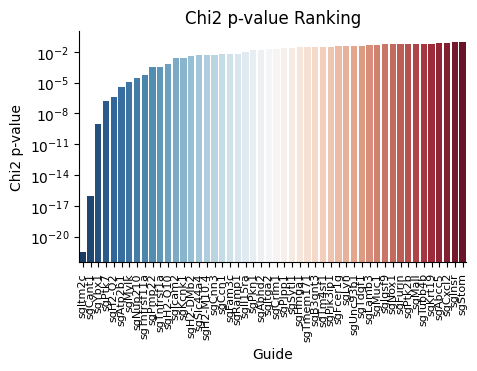
spc.rank_by_chi_square(fdata, cluster_field='nmf_cluster')
spc.plot_ranking_bar(fdata, 'Chi2 p-value')
The result is shown below.
This function plot_ranking_bar() is a simple function to plot the chi-square test result using bar plot.
An alternative visualization is shown below.
This function plot_ranking_scatter() is a simple function to plot the chi-square test result using scatter plot.

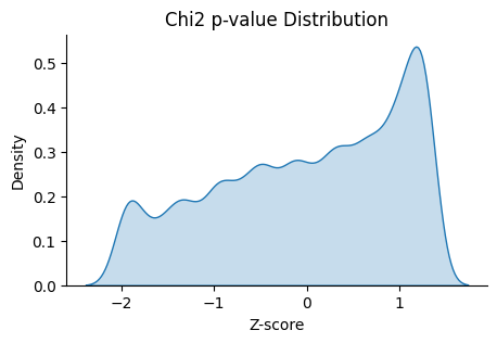
We can also check the distribution of the guides with low Chi2 p-value.
This function plot_ranking_hist() is a simple function to plot the chi-square test result using histogram
to demonstrate the distribution of the guides with low Chi2 p-value.
Note
Chi-square test ranking requires clustering information. Make sure to perform clustering on your data first. The test evaluates whether guides show significantly different patterns across clusters compared to the control.
All chi-square test results are stored in the adata.uns attribute named ‘Chi2 p-value’ by default.
Before we can move on to cluster independent analysis, we can try identifying the guide’s specificity in a particular cluster.
SPOT provides a function sp.cluster_independent.volcano_plot() to perform chi-square test on a particular cluster for each guide,
determining the specificity of each guide in the cluster.
Similar to RNA-seq analysis, we can perform volcano plot to visualize the guide’s specificity in a particular cluster.
sp.cluster_independent.volcano_plot(fdata, cluster_field='nmf_cluster', cluster_id=0)
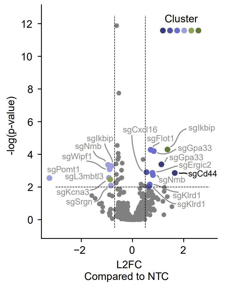
In this plot, the x-axis is the guide’s specificity in the cluster, and the y-axis is the -log10(p-value) of the chi-square test. The gray lines is the threshold of the p-value, and the guides with p-value less than the threshold are considered to be specific to the cluster. Colored dots are the guides with p-value less than the threshold, meaning their specificity is significant in the cluster.
For instance, in the plot above, we can see that the guide ‘sgCd44’ is specific to the cluster marked with dark blue color, meaning enrichment.
Note
The threshold of the p-value is set to 0.05 by default. You can change the threshold by setting the threshold parameter.
Cluster Independent Analysis
In cluster independent analysis, we perform KL divergence test to determine the guide specificity compared to non-targeting guide. Cluster independent means that we would like to know the guide specificity compared to wild type T cells.
More detailed information about modeling can be found at [our paper](https://www.nature.com/articles/s41592-024-02012-z).
Note
KL Distance Ranking is generally a method to model distribution of guides that have low spatial resolution or the spatial encoding is not the essential feature. As KL Distance Ranking dicards the spatial relationship between locations.
import sp.cluster_independent as spc
spc.rank_by_relative_entropy(fdata, reference_guide='sum')
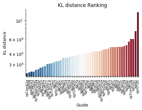
spc.plot_ranking(fdata, 'KL distance')
The result is shown below.
This function plot_ranking() is a simple function to plot the KL divergence test result using bar plot.
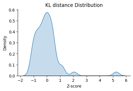
We can check the distribution of the guides with high KL distance.
This function plot_ranking_hist() is a simple function to plot the KL divergence test result using histogram
to demonstrate the distribution of the guides with high KL distance.
All KL distance results are stored in the adata.uns attribute named ‘KL distance’ by default.
Warning
KL divergence test requires reference guide. Make sure to set the reference guide correctly using the reference_guide parameter. The reference guide can be set to ‘sum’ or ‘ntc’ (non-targeting control guide).